

Slides: Tiering adjustment_FINAL
pdf: How was tiering facilitated_FINAL
On 30th October, the European Central Bank’s (ECB) new tiering system came into operation, resulting in the reshuffling of liquidity across the Eurosystem. As noted previously, and reported variously, this caused a record one month decline in Italy’s TARGET2 debit, falling EUR48bn to reach EUR420bn—the lowest debit for 2 years. At that time this blog speculated the introduction of tiering created an arbitrage opportunity, allowing Italian banks to draw in liquidity to deposit at 0%. As liquidity was returned to the periphery, TARGET2 balances adjusted.
This hasty “interbank” interpretation of adjustment was reasonably challenged—on twitter and elsewhere. Indeed, at the time it was noted how “other sources of funding” might provide an alternative explanation. And, over the past few weeks, further data allow a more nuanced interpretation of this adjustment. Moreover, a recent piece by the ECB confirms a key role played by collateralized lending in this process. Here we therefore contemplate again this adjustment.
Various data shed light on evolving Eurosystem balances. Daily data on aggregate liquidity; weekly data on the Eurosystem and Bundesbank balance sheets; 6-weekly snapshots of the disaggregated Eurosystem National Central Bank (NCB) balance sheets reported by the ECB, amongst others. We begin recalling the pre-tiering snapshot on the distribution of Eurosystem liquidity.
Snapshot: Early-October
Figure 1 shows ECB data on the distribution of deposits—current account and deposit facility, or “total liquidity”—as of 4th Oct, 3½ weeks before tiering.

Total liquidity was predominantly held on current account with respective NCBs—largely in Germany (EUR617bn) and France (EUR467bn) where 58% of the aggregate 1,864bn held by respective monetary financial intermediaries (MFI) was kept. Against this, not shown, withdrawn from availability as reserves in the aggregate was EUR269bn held by governments, EUR138bn by other non-MFI intermediaries, and EUR230bn by non-residents. Beyond the redistribution of reserves, these provided alternative sources of liquidity for MFIs to fulfill tiering.
Total deposits relative to required-plus-tiered reserves (Figure 1, right side) reveals a number of countries’ banks were, as of 4th Oct, short of the liquidity needed to exploit tiering. A ratio of 1 implies enough reserves already available within the domestic banking system—not necessarily distributed suitably within the country, of course. While the aggregate ratio was 1.85, country level aggregates from Ireland down point to fewer reserves—and banks in Portugal, Slovakia, Italy, and Greece, at less than 1, were short of the amount needed to meet local tiering possibilities without drawing upon reserves from abroad or elsewhere.
Daily data: Aggregate liquidity
Figure 2 shows system-wide excess liquidity from 4th Oct—defined as total liquidity minus required reserves. Driven by “autonomous factors and monetary policy portfolio” (AF) flows, excess liquidity fell roughly EUR45bn, from EUR1,730bn to EUR1,685bn, before increasing sharply during the days immediately before tiering came into effect. Thereafter, excess liquidity further increased to EUR1,815bn on 8th November—the highest stock since mid-June.
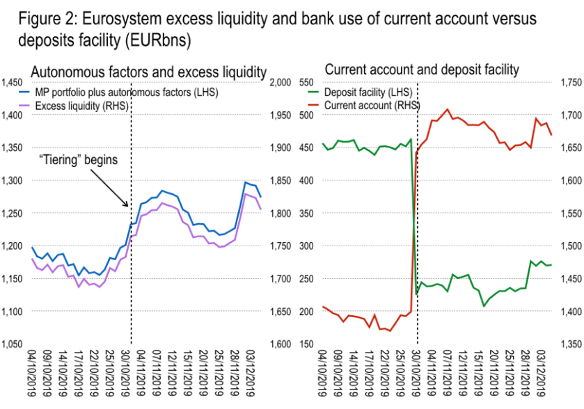
Meanwhile, within excess liquidity can be witnessed a last-minute switch from the deposit facility to current accounts. Indeed, the deposit facility fell about EUR240bn on 30th Oct, when current accounts increased roughly the same amount. Over the following week, liquidity held at banks’ current accounts with the ECB increased a further EUR65bn before rolling off along with AF.
Liquidity held in current accounts prior to 30th Oct was already more than enough to satisfy the system’s aggregate required-plus-tiered reserves. The last-minute switch from deposit facility is perhaps another expression of asymmetric intra- and inter-country liquidity distribution.
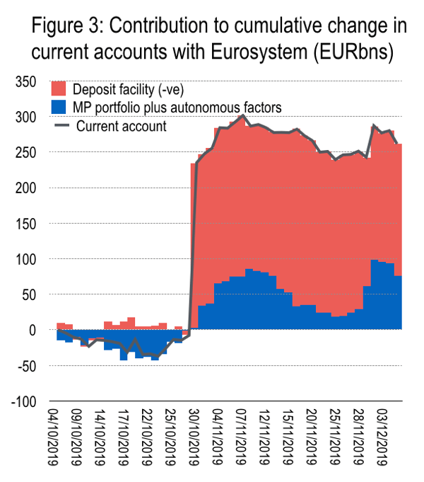
The contributions of AF and the deposit facility to the cumulative change in current accounts since Oct 4th is shown in Figure 3. AF withdrew liquidity before liquidity was added around the time tiering came into effect.
Weekly data: Adjustment to tiering
Further information is provided by Bundesbank and Eurosystem aggregate balance sheets—weekly snapshots available every Tuesday for the preceding Friday.
Figure 4 shows total liquidity in Germany and the rest of euroarea (ROEA.) The axes are different, but the scale on each is EUR140bn. Liquidity in Germany began on 4th Oct around EUR620bn, trending down to about EUR580bn on 22nd November; through 25th Oct falling EUR24bn. Over the period through 8th Nov, liquidity in Germany was largely unchanged. Initially total liquidity in ROEA shrank before increasing sharply—during the three weeks from 18th Oct and 8th Nov by EUR23bn, EUR50bn, and EUR28bn respectively, a total of EUR101bn.
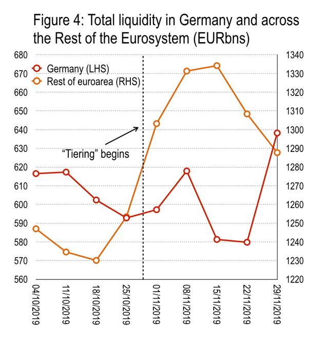
Over the crucial period leading up to tiering on 30th Oct, between 4th Oct and 1st Nov, liquidity in Germany fell EUR19bn while ROEA saw liquidity increase EUR56bn.
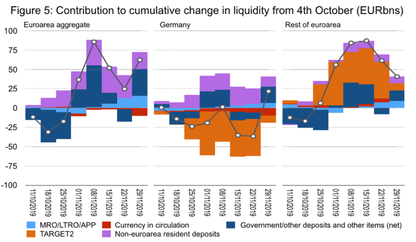
Figure 5 decomposes the cumulative change in liquidity over this period into the main balance sheet items. After falling initially, total liquidity increased sharply into the first two weeks of Nov in the aggregate (left panel). The two main drivers were government and other deposits (about 2/3rds) and non-resident euro deposits (about 1/3rd).
However, the drivers in Germany (middle panel) versus ROEA (right panel) were different. As noted above, the cumulative change in total liquidity in Germany through 8thNov was roughly zero. However, there were contributions to liquidity of EUR23bn by government and other deposits, and from non-euroarea residents of EUR21bn. Against this, Germany’s TARGET2 credit contracted EUR40bn through 8thNov (and EUR56bn through 1stNov.)
The counterpart to these flows, of course, was largely a decrease in TARGET2 debit of ROEA—the mirror of Germany’s credit. Onto this was a contribution to liquidity from government deposits and non-euroarea resident deposits.
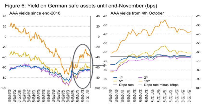
As noted previously, non-euroarea euro deposits represent reserve manager euro claims yet to be allocated to securities. In a sense, they represent asset purchase program (APP) purchases by the Eurosystem from non-resident central banks that have yet to be re-deployed. Thus, it represents a liquidity buffer. The interest on these deposits at the Bundesbank are the deposit rate minus 15bps, so since September -65bps. And if the front end of the safe asset euro yield curve provides a negative rate below this, absent a change in attitude to risk, reserve managers should just keep these euros as deposits with the Eurosystem. But once the front end of the yield curve touches -65bps, there is an incentive for these deposits to be rundown and rotated back into securities once more. This provides a cap on the front end of the bund yield curve.
Figure 6 shows the daily yield on AAA securities in Germany reported by the Bundesbank. Yields were pushed ever lower across the curve throughout the course of 2019. A snapback in yields accompanied the September ECB meeting—arguably markets were hoping for a more aggressive rate cut by Draghi. By the first week of October (right panel) 1-5Y yields were consistently below -65bps. But during the week preceding 25th Oct, yields moved higher—coincident with the decline in Germany’s TARGET2 credit. This would be consistent with bund sales by non-Core banks preparing for tiering, dragging yields higher until non-resident reserve managers in turn were dragged back in as the yield touched -65bps.
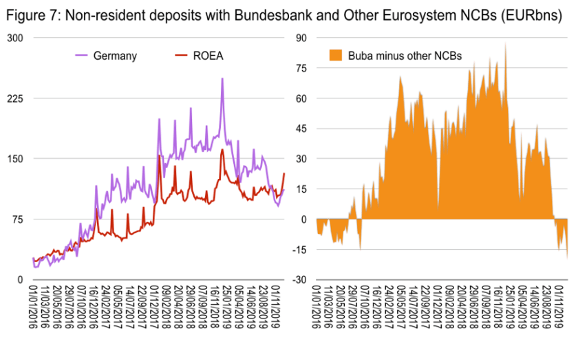
Indeed, the inflow from non-resident deposits of 23bn during October helped bring non-resident deposits with the Bundesbank below those held across the rest of the Eurosystem for the first time since 2016. Figure 7.
Monthly data: Which countries drew on external resources?
It might be expected that countries with TARGET2 credits prior to tiering, like Germany, might witness capital outflows while debit countries inflows in the run up to tiering. Figure 8, using the 4th Oct and 1st Nov balance sheet data from ECB, shows how this simplistic view is misleading. The chart shows the initial TARGET2 position and the change over this period for 9 major economies. If all creditors to the system saw capital outflows, and all debtors inflows, the chart would show balances moving in a clock-wise direction. Indeed, while Germany (-EUR57bn) and Italy (+EUR69bn) are consistent with this view. However, some creditors—such as Finland Luxembourg—saw inflows and larger TARGET2 debits post-tiering. Meanwhile, Spain saw outflows despite beginning with an initial debit balance. Belgium and France started near zero initial TARGET2 position and each saw outflows.

Figure 9, finally, decomposes the contributions to the change in current accounts for these same countries over the same period. In very case the deposit facility was drawn down (a positive contribution) to top up current accounts. As noted above, the TARGET2 system saw some countries accumulate liquidity flowing from Belgium, France, Germany, and Netherlands. Meanwhile, German liquidity benefitted from inflows by non-resident reserve managers.
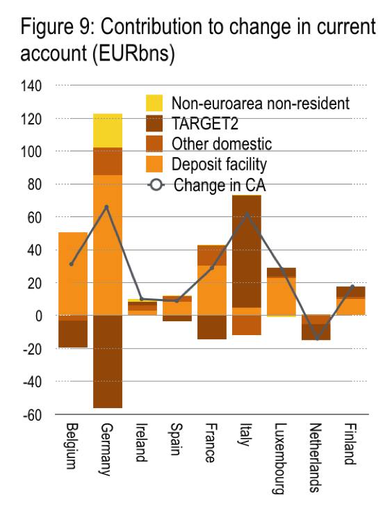
END.
